VH-1 is based on the description of the piece-wise parabolic method (PPM) given in Colella and Woodward (J Comp Phys, 1984; hereafter "CW"). Here we present a brief overview of VH-1, starting with the system of equations that it solves, the finite volume approach to numerical solutions, and the Lagrange-Remap version of the Piece-wise Parabolic Method. This is only a cursory introduction to PPMLR. For further details please read CW.
Euler Equations
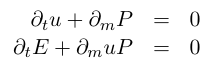
VH-1 uses finite difference techniques to solve the Euler equations of ideal inviscid compressible gas flow. These equations, written in conservative, Eulerian form are:
These equations represent the conservation of mass, momentum, and energy, respectively. The primary variables are the mass density rho, gas pressure P, and fluid velocity u. The total energy per unit mass is the sum of the kinetic energy and the internal energy:
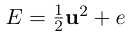
and the internal energy is related to the pressure through the equation of state for an ideal gas:
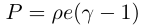
The only source term included here is a local acceleration, a, such as that due to gravity. VH-1 does not include an energy source term, but such a term can be readily added using an operator splitting method. Because an acceleration term is already present in the form of fictitous forces for a curvilinear grid, we have included an arbitrary acceleration term in VH-1.
Finite Volume Representation
Representation on a finite grid, definitions as volume averages, replacing derivatives with finite differences, boundary conditions, Courant limit on timestep.
PPMLR
VH-1 is written as a one-dimensional Lagrangian hydrodynamics code coupled with a remap onto the original Eulerian grid. Two or three dimensional problems are reduced to one-dimensional updates using operator splitting. Thus the fundamental building block of VH-1 is a one-dimensional update of the Lagrangian fluid equations followed by a conservative remap. This implementation of PPM is referred to as PPMLR.The following is an outline of the PPMLR algorithm. For specific details see CW. As an illustration, let us consider the equations of ideal hydrodynamics in Lagrangian coordinates in one dimension, planar geometry and no source terms. Written in conservative form these equations are:
These conservation equations can be finite differenced as:
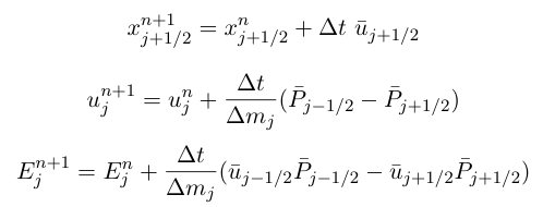
where the subscript j refers to zone averaged values, and subscripts j-1/2 and j+1/2 refer to values at the left and right hand sides of the zone, and the superscript is the timestep.
The variables u-bar and p-bar are the time-averaged values of the velocity and pressure at the (Lagrangian) zone interfaces. The trick is clearly to obtain accurate, stable estimates of these quantities.
The approach of Godunov's method is to obtain these time-averaged quantities by approximating the flow at each zone interface during each timestep with a Riemann shock tube problem. At the beginning of the timestep, the zone interface is modelled as a discontinuity separating two uniform states given by the zone averages on the left and right side of the zone interface (zones i-1 and i). This constructed Riemann problem is then solved to find the time-averaged value of the velocity and pressure at this discontinuity (zone interface), u-bar and p-bar. The solution of the non-linear Riemann problem typically requires some kind of iterative procedure, as described in van Leer (1979) and in Woodward (1986).
PPM improves upon this method by using more accurate guesses for the input states to the Riemann problem (the values on either side of the interface). Using a quadratic interpolation of the fluid variables in each zone, the Riemann input states are taken to be the average over that part of the zone that can be reached by a sound wave in a time dt, i.e., the characteristic domain of dependence.
Once the hydrodynamic equations have been differenced to obtain the values at t+dt, the fluid variables can be instantaneously remapped from the Lagrangian coordinate system to the stationary Eulerian grid. This remap step uses the same quadratic interpolation method that was used in the hydrodynamics step.
This description makes PPM sound relatively simple, but there are many key ingredients that we have skipped over, including the parabolic interpolation and monotonicity constraints, the iterative Riemann solver, and additional dissipation mechanisms. We will give a brief discussion of these first two topics in the appropriate subsections of Chapter 2 and postpone the discusion of dissipation until Chapter 4 (see also CW).