INTRODUCTION
In this lesson we will study numerical solutions to
Laplace's Equation,
which represents a class of partial differential equations known as elliptic equations. We will use a simple, robust method known as the relaxation method. We will discover, however, that for large problems (many points per dimension), the relaxation method becomes very inefficient. In this case there are other, more efficient methods for solving elliptic PDEs.
Laplace's equation arises in many contexts in physics, but the most common problem is that of static electric fields. If you open up your electrodynamics textbook and look on the inside cover, you will probably find a listing of the four Maxwell's equations. For a static problem with no electric charges, the first of these equations looks like
If there are charges present (in which case the equation is known as Poisson's equation), one approaches the problem in a similar manner, but we will save this complexity for the next lesson. If we rewrite this in terms of the electrostatic potential we get Laplace's equation:
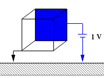
As an example, let us consider the problem of finding the electrostatic potential inside a cube in which 5 of the 6 sides are held at zero potential, and one side is held at 1 Volt.

Rather than jump right into this problem, lets go one small step at a time, beginning with a one dimensional problem. Remember the electrostatics of a plane-parallel capacitor? If the two plates are a small distance apart, we can neglect the edges and assume the potential depends only on the coordinate between the plates.
In one dimension Laplace's equation reads
and the solution is
This is nothing more than the equation of a straight line. The integration constants are given by the boundary conditions of the problem, e.g., by the potential on both ends of our one-dimensional "space." If we impose the boundary conditions that one side of our 1D 'box' at a position x = 0 is at a potential of -1 Volt and the other side at a position of x=L is at +1 Volt, what is the solution for the potential inside our 1D box? [What are the values of m and b?]
While the solution to Laplace's equation in one dimension is indeed very simple, it serves to illustrate some key points.
- First, the solution at any one point is given by the average of neighboring points.
- Second, the solution on the interior is always bracketed by the solution on the boundaries.
- Third, there is only one solution matching the appropriate boundary conditions.
The relaxation method derives from these properties, noting that the potential at any point on the one-dimensional grid will be given by the average of it's two neighbors
To appreciate the relaxation method for solving this equation, we first note that Laplace's equation looks very similar to the diffusion equation:
In fact, if we evolve the solution V(x,t) ahead in time until it reaches a steady-state (such that the time derivative equals zero), we have found the solution to Laplace's equation. The relaxation method is then nothing more than the finite-difference solution to the diffusion equation.
Finding the solution to Laplace's equation involves iterating this equation many times (evolving the solution to the diffusion equation forward in time). We learned previously that this numerical method is stable only if the time step is smaller than (or equal to) the maximum value given by
If we use this limiting value, our numerical solution looks like
Note that this equation gives the solution at coordinate i as the average of the solution at i+1 and at i-1, in accord with the first property of Laplace's solution listed above.
The relaxation method is then nothing more than evolving this finite-difference version of the diffusion equation forward in time until the solution reaches a steady state. At this point the potential, V(x), has "relaxed" to the unique solution to Laplace's equation and the potential at any point is given exactly by the average of its two neighbors.

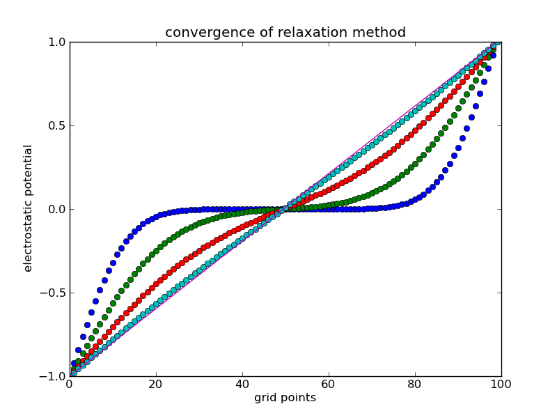
A numerical solution to the one-dimensional Laplace equation would look like the following:
- Declare a 1D array to store the electrostatic potential, V(nx)
- Set the boundary conditions (these values are fixed by the problem)
- V[0] = -1 (first number in array)
- V[nx-1] = +1 (last number in array)
- Iterate the relaxation equation many times for each point on the grid
- V[i] = 0.5 * (V[i-1] + V[i+1])
- Compare the final solution with the correct answer (a straight line)
Exercise: Write a program to solve the 1D Laplace equation for a given set of boundary conditions. Plot out the solution for different numbers of iterations. Qualitatively speaking, how many steps are needed to reach a "good" solution?

The figure above shows the solution, V(x), after 100, 200, 400, and 800 steps. From this we can see that after 800 steps the solution is close the the anticipated straight line, but to be useful we would like to have some means within the program of knowing how many steps are needed to reach the correct solution. Of course this brings up the question of how correct is correct!
One might rephrase this question to ask how many iterations are needed such that the solution does not change by more than 0.1% in a timestep. Lets try to answer this question by adding some code to keep track of the average change in potential at each iteration:
Vold = V.copy()
for i in range(1,nx-1):
   V[i] = 0.5 * (V[i+1] + V[i-1])
u = (V - Vold)
err = sqrt(dot(u,u))
This is not a very practical approach because the value of err corresponding to a given accuracy of the solution depends strongly on the number of zones in the grid. In our case we know the exact solution, so we can instead sum up the difference between our iterated solution and the true solution.
Vtrue = linspace(-1.,+1.,nx)
u = (V - Vtrue)
err = sqrt(dot(u,u))
We can then use this error calculation and have the relaxation method iterate until the error drops below some specified value, say 0.1%.

Before proceeding further, lets make use of numpy to make our code much faster. If you are using a for loop to loop over your 1D grid, you can speed up your code significantly by using numpy's intrinsic indexing. The following loop over the interior of the grid (not touching the two end points representing the boundary conditions
for i in range(1,nx-1):
   V[i] = 0.5 * (V[i+1] + V[i-1])
can be replaced by the single statement
V[1:-1] = 0.5*(V[:-2] + V[2:])
which states that nx-2 values of V from 1 (the second value since the first is index zero) to the (last minus 1) value are to be replaced with the average of the values from the first (default, since nothing specified) to the (last minus 2) and the values from the third to the last (default). How much faster does your code run with this line replacing a for loop?

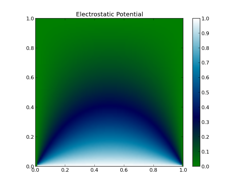
Assignment: Compute the electrostatic potential for a two-dimensional box with 3 sides fixed at zero potential and one side fixed at +1V.

This image was created with
imshow(V, extent=[0,1,0,1], cmap='ocean')
colorbar()
A list of available colormaps is available at matplotlib.org.