INTRODUCTION
In this lesson we will use the Ising model to investigate the concept of a
phase transition.
Specifically, we will study the second-order, or continuous phase transition
in the Ising model, representing the transition between a magnetized and an unmagnetized
state of a ferromagnetic material.
We begin with the code from the last lesson, which computes the bulk magnetization of a 2D lattice as a function of the 'Monte Carlo time', defined as the number of complete passes of spin flips over the lattice.
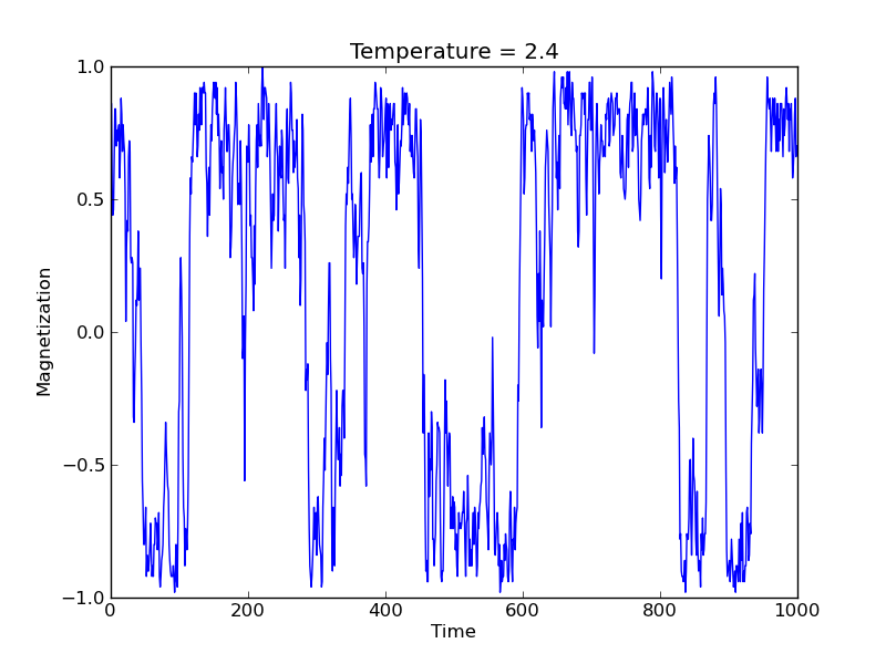
This system exhibits a phase transition between a fully-aligned lattice where all the spins are oriented in the same direction, and a lattice of randomly-aligned spins. The former happens when the temperature is low and there is insufficient thermal energy to flip a spin that is already aligned with its neighbors. The latter happens when the average thermal energy is more than sufficient to flip any spin in the lattice. In terms of the time average of the bulk magnetization, the cold, aligned state would have a bulk magnetization of unity, and the hot, un-aligned state would have a bulk magnetization near zero.
We can illustrate this transition by adding an outer loop over temperature, and plotting the average magnetization versus temperature:
for k in range(35):
  temp = temp + 0.1
  for n in range(steps):
      ### Monte Carlo evolution ###
      mag = sum(spin) / numberofcells
  magnetization[k] = average(mag)
  temperature[k] = temp
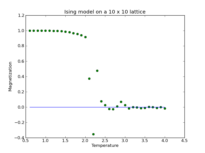
Averaging the magnetization over more passes through the lattice will decrease the scatter in this plot (the above plot used 1000 passes), but not necessarily in the vicinity of the transition temperature where one sees dramatic swings in the bulk magnetization.
In the study of thermodynamics, one often interprets phase transitions in terms of the behavior of the free energy of the system as a function of other thermodynamic variables. To gain further insight into the phase transition seen in our Ising model, we can look at the average energy per spin in the lattice:
where the summation is over N microstates $\alpha$ of the lattice generated by the Monte Carlo simulation. The energy of a given microstate is given by a sum over all pairs of neighboring spins (but be careful to only count each pair once). At low temperatures all the spins are aligned, so each pair of spins contributes an energy of -J (where we have been using J=1 in our code). Each cell in the lattice has four neighbors, but dividing by two to avoid double-counting each pair, we expect an average energy per spin of -2J. At sufficiently high temperatures we would expect the spins to be truly random. In this limit the average energy should approach zero, as each spin would have two spins aligned and two mis-aligned. The fact that the computed energy is still significantly below zero for temperatures used in our models suggests that the neighboring spins are still correlated even though the bulk magnetization averages to zero.
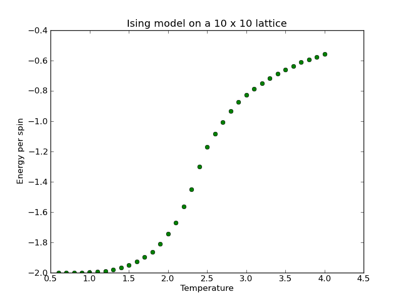
Assignment: Compute the energy per spin as a function of temperature, as shown above, illustrating the phase transition of the 2D Ising model.
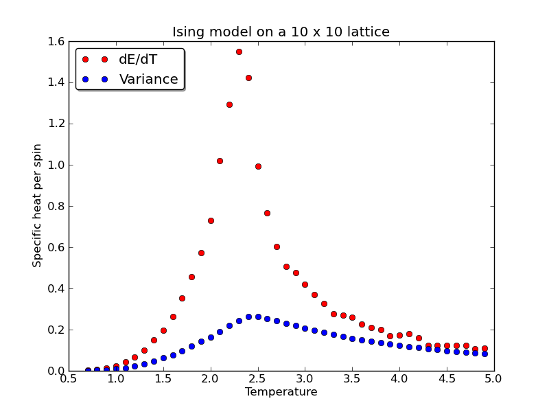
The phase transition studied here is known as a second-order phase transition because the second derivative of the free energy is discontinuous. The first derivative is continuous as shown in the plot above, but it exhibits an inflection point. As the lattice size is increased, the slope at the inflection point increases. In the limit of an infinite system, this slope becomes infinite.
The slope in this plot is known as the specific heat. For a large system, a second-order phase transition is thus characterized by a divergent specific heat. What does this tell you about the energy needed to heat the system up past the transition temperature?
Taking a numerical derivative of the data shown above gives us:
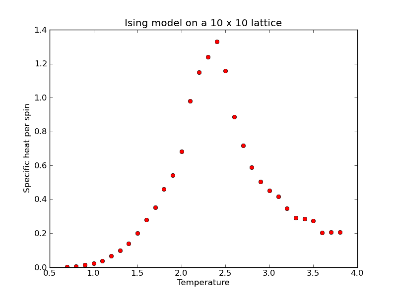
This same divergent behavior can be seen in the variance of the energy of the system. These two quantities, the variance and the specific heat, are related by the fluctuation-dissipation theorm. Try making sense of this theorem by reading the wikipedia entry (Hah!). For our purposes, the FDT gives us another way to compute the specific heat:
where the variance of the energy is defined as:
Assignment: Compare the two definitions of specific heat per spin as a function of temperature.
