Random Systems

INTRODUCTION
The application of numerical methods to solve a set of differential equations describing a deterministic physical phenomenon is an obvious application of computational physics. A less obvious application is the use of computers to study random processes. In many cases the exact, deterministic solution of a physical problem is far too cumbersome to handle analytically or numerically. To simplify the problem we describe it in terms of random processes.

Consider, for example, the propagation of a photon out of the core of the sun. The interaction of the photon with the hot plasma in the Sun's core can be described by a set of differential equations that can in principle be solved with techniques we have discussed previously. However, even for one photon, this calculation would be impossibly large given that a typical photon in the core of the sun travels less than a centimeter before it scatters off an electron. Keeping track of the 10⁵⁷ electrons in the sun, as well as the lone photon we are tracking, and computing the electromagnetic interaction of the photon and all those electrons is out of the question. Instead, we can approximate the problem with a statistical process, neglecting the details of each scattering.

In addition to studying physics with a statistical approach, one also finds frequent use of random numbers in less obvious situations, such as computing multi-dimensional integrals. At the heart of all these random techniques is a random number generator. Most programming languages come equipped with access to a random number generator - some function that when called from your program will return a random number between 0 and 1. Note, however, that one should always be cautious when using random number generators; not all random numbers are "equally random." As usual, Numerical Recipies provides some valuable insight into this topic. For our purposes, the random numbers provided by the system routine will be sufficiently random.

In Python the function call random() will return a real value between 0 and 1. You can generate an array of random numbers all at once by passing this function an integer:

In [4]: from matplotlib.pylab import *

In [5]: random((5))
Out[5]: array([ 0.68031985,  0.95085031,  0.88318264,  0.45968826,  0.15139228])

Exercise: Plot a histogram of an array of random numbers. In this example 1000 random numbers are sorted into 10 bins:

hist(random(1000),10)
show()

Compare the deviations from a uniform distribution as a function of the number of random numbers binned.

Monte Carlo

Monte Carlo methods are a group of numerical methods that use random numbers to investigate a problem statistically. Take the example from the last lesson of a photon diffusing out of the Sun. We could model this diffusion process as a random walk (which we will study later this lesson), using random numbers to calculate the path of a single photon bouncing it's way out of the Sun. If we repeated this process for a large number of photons, we could gather statistics on how long it takes photons to get out of the Sun. If we went back and added more physics into our model, e.g., calculating the changes in photon number and energy with each collision, we could also gather statistics on the spectrum of photons emerging from the Sun.

Another practical application of Monte Carlo is in the evaluation of multidimensional integrals. The basic idea of Monte Carlo Integration is to statistically sample some known volume (for a 3D integral) and find the fraction of that volume that falls inside the integrand. The common analogy is that of a dart board. Consider the following integral for the area of a circle:

The Monte Carlo approach would be analogous to throwing darts randomly (but uniformly!) at a known area that encompasses the dart board, e.g., a square with width equal to the diameter of the dart board. The area of the dart board should equal the area of the square times the ratio of the darts that hit the board to those that miss:

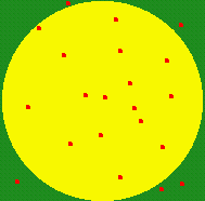
Clearly, the more darts you throw, the more accurate your answer will become. Our first step is to write down an algorithm to describe the steps a program would perform in order to do this integration:

1. Choose a known area to throw darts at (e.g., X and Y limits of a rectangle)
2. Throw many darts at random locations and record results
   1. Use random() to pick random x and y
   2. Test to see if dart is inside our target area (in this case, when R < 1)
   3. If the dart hit the target, add it to the counter
3. Calculate area of dart board from area of square

Exercise: Use the Monte Carlo Method to compute the area of a circle of unit radius (pi!).

Since this is a statistical method, it is not expected to give an 'exact' answer, nor is it going to give the same answer every time. As such, the accuracy itself is only a statistical parameter. If we were to repeat this area calculation many times with different random distributions of darts, we would get different answers each time. The distribution of answers would be centered on the correct value, but with a width that depends on the number of darts thrown. The graph below shows the distribution of 500 separate calculations, with each calculation involving 10,000 or 100,000 random points. Using more darts produces a more sharply peaked distribution, such that one is more likely to get the correct answer.

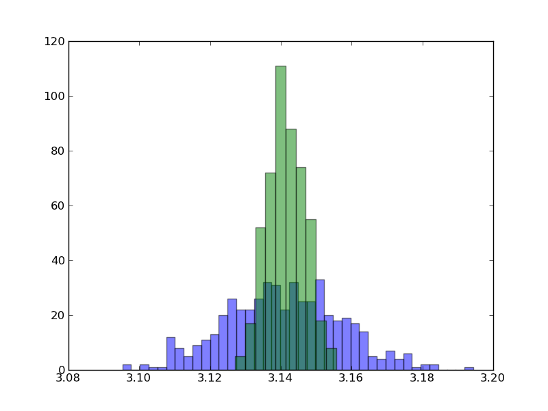
The power of Monte Carlo integration is that the error, given by the width of the distribution in the above plot, scales with the square root of the number of darts thrown, independent of the number of dimensions in the integral. In contrast, the standard numerical integration methods we saw in earlier lessons have an error that scales with some power of the number of points in each dimension. For example, for a one dimensional integral, the error in Simpson's rule scales as N^-2. This is much better than the error scaling in the Monte Carlo method because the error becomes smaller with increasing N much faster with Simpson's rule. However, for an integral over D dimensions, Simpson's rule must split up the points over the D-dimensional space, such that there are only N^1/D points per dimension. The error with Simpson's rule then scales as N^-2/D. This becomes inferior to the Monte Carlo method for D > 4. Thus, physicists often turn to Monte Carlo Integration when dealing with integrals in many dimensions.

Distribution Functions
In statistical physics one often wants to model a distribution of objects (e.g., molecules) that are described by some distribution function. A common example is the Maxwell-Boltzmann velocity distribution:

where $P(v) dv$ is the probability that a moledule of mass m has a speed in the range $v$ to $v + dv$. Note that aside from the mass of the molecule, the only parameter in this equation is the temperature of the gas. The problem is how do you turn a uniform distribution as provided by random into a something like the Maxwell-Boltzmann distribution? The simplest approach is known as the rejection method.

Our problem is this: We want to get random values of v such that the probability of picking a value between v and v + dv is given by the function P(v).

First, pick the desired range of v from which we will draw random values: v_min, v_max.

Second, find the maximum value of P(v) for the chosen range of v: P_max.

Finally, we can pick random values of v through a two-step process:

1. Use random() to pick a (uniformly distributed) random number, v, between v_min and v_max
2. Use random() to pick a probability, p, between 0 and P_max
3. If p is greater than P(v), reject this value and try again

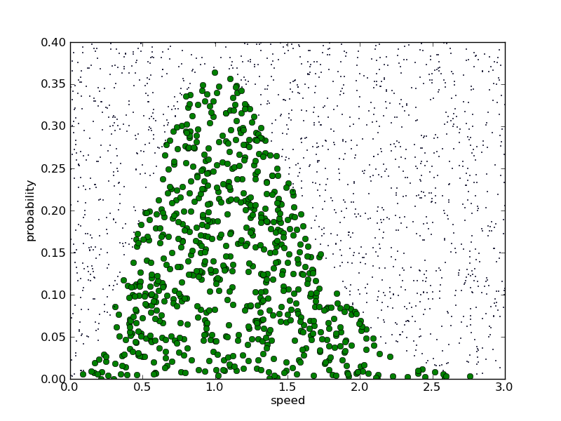
You can think of this as a two-dimensional random process where you pick a random v and p within a prescribed rectangle. If your random point falls under the desired distribution function, keep it. Otherwise, throw it away. Note that if your distribution function was sharply peaked, you would be throwing away alot of random numbers. In this case, it would be more efficient to chose your random point not from a rectangle, but from some other shape (see Numerical Recipies for a more efficient version of the rejection method).

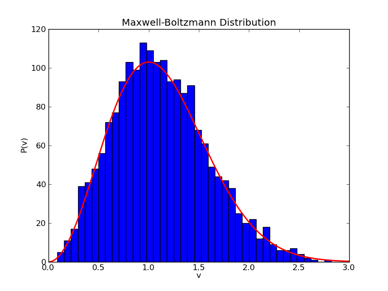
Assignment: Write a code that chooses random velocities that satisfy the Maxwell-Boltzmann velocity distribution. Plot a histogram of your random values and plot the results along with the analytic Maxwell-Boltzmann distribution function, as shown below.