INTRODUCTION
Fourier analysis is a powerful tool in physics, and in particular in computational physics.
This is often true when dealing with a time series, such as generated in the last few lessons
on chaos. One is often asking, what is the dominant frequency in this system? You can look
at a plot of the time evolution and you can 'see' periodicity, but how do you quantify it?
We begin with the basic concept that a function can be represented by a linear combination of harmonic functions:
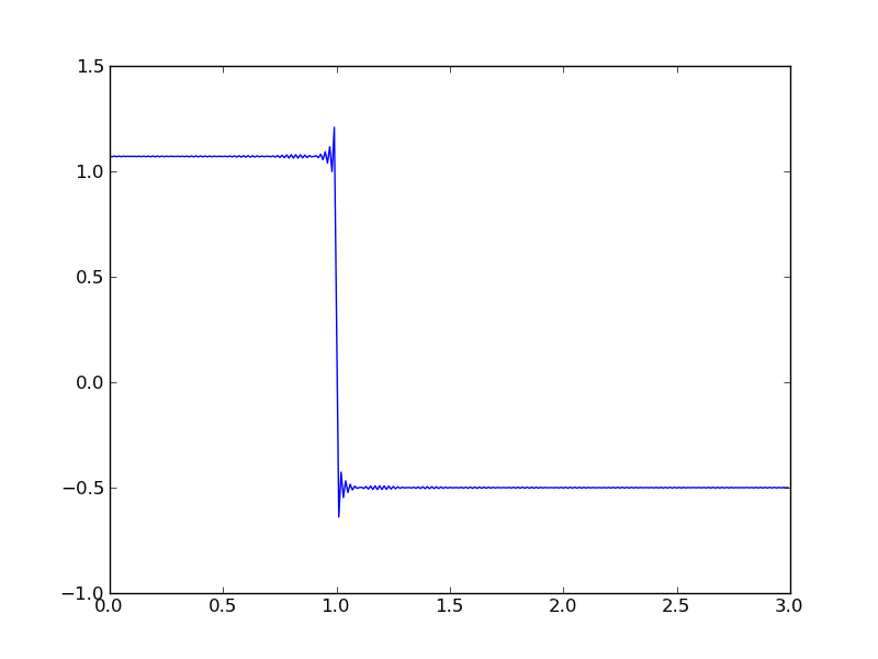
As a specific example, consider the series
Exercise: Write a python program that adds up the terms in the series above. Changing the value of N, compare your result with the plot below and estimate how many terms were used in this plot.

A more convenient way to express the first equation, in the continuum limit, is
Here the coefficients are now represented by a continuous function, Y(f), known as the Fourier Transform. Note that by replacing sine and cosine with an exponential through Euler's formula, we now must contend with complex numbers. The inverse of this expression is
A Discrete Fourier Transform arises when we only know values at discrete points, as typically happens in compuational work. For example, if we know the value of some function y(t) at discrete time intervals separated by a time step $\Delta$, i.e., we know the values of $y_j = y(j\Delta)$, the Discrete Fourier Transform would look like:
where $Y_k$ is the Fourier amplitude at the discrete frequency $f_k = k/(N\Delta)$. One of the reasons for the widespread use of Fourier Transforms in computational physics is the existence of a very efficient algorithm known as the Fast Fourier Transform, or FFT. As with most useful things in computational physics, there is a built in function in SciPy to compute FFTs.

Fast Fourier Transforms
To explore this function and what it can be used for, lets start by generating the
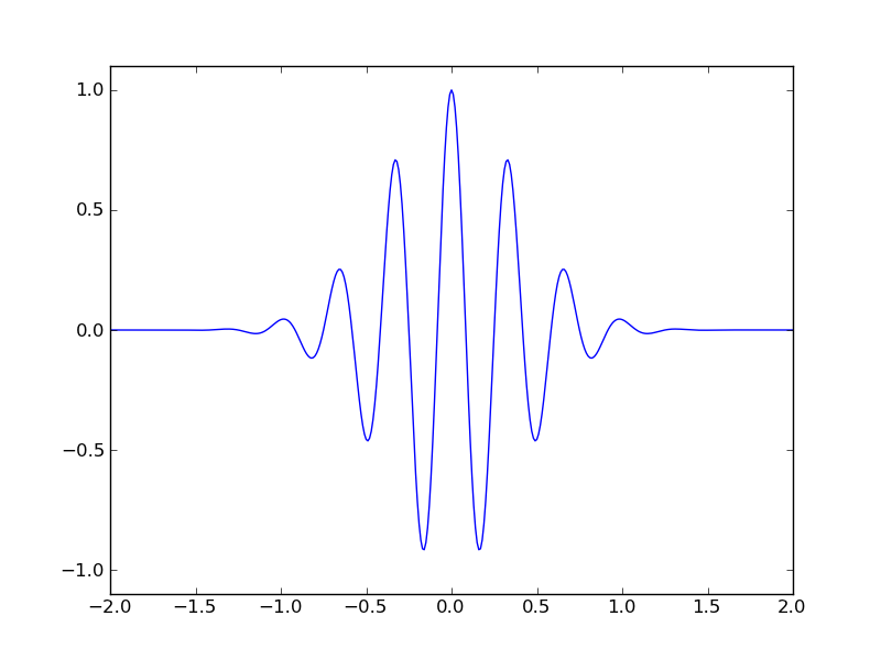
function used to illustrate Fourier Transforms on the Wikipedia page.
First, generate the function in a python program (plot it!):

The next step is easy: Y = fft(y). If you plot just this function you will get something a little strange. First of all, there are two identical traces. This stems from the fact that the formal transform returns both positive and negative frequencies, but if the input signal is real-valued, these two halves of the transform are identical. In this relatively common case, you can use the python function rfft instead, which returns just the positive frequencies. But what are those frequencies?
Second, note that Y is complex. Plot the real part with Y.real and the imaginary part with Y.imag. Lest you think the imaginary part is small and can be ignored, change your input function from a cosine to a sine. What happens to Y?
Note that if our original function has N data points, the rfft function returns N/2+1 frequencies. Using our definition for $f_k$ above, these frequencies range from zero to the Nyquist frequence
If the input signal was a simple sine wave at the Nyquist frequency, it would only have data values recorded twice per period. Any higher frequency is not 'detected' by this procedure. Moreover, the power in frequencies higher than $f_c$ will be aliased to lower frequencies, providing false results.
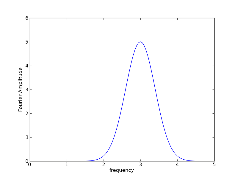
To make our transform plot complete, we need to generate an array of frequencies from zero to the Nyquist frequency. The result should look like:

Note that the peak is right at f=3Hz, in agreement with our input function y(t). How does your transform depend on the choice of $\Delta$? Does it depend on the time limits of your input data? Why or why not?

Power Spectral Density
The last step is to generate a power spectrum or periodogram - an estimate of the spectral density.
This represents the power in a given frequency. The power is nominally just the square of the
amplitude - but how do you account for the fact that Y is complex?
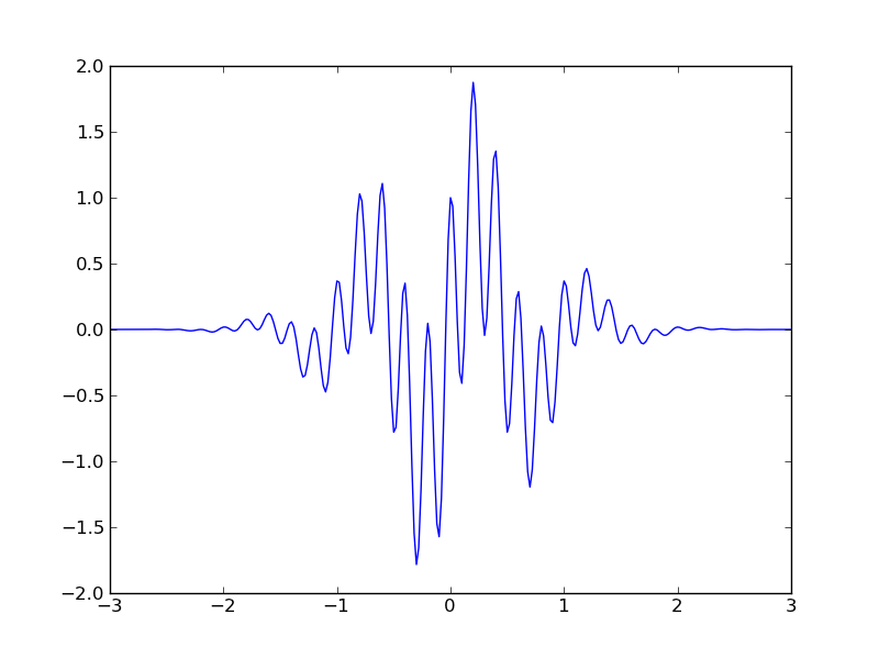
Assignment: Download this dataset and generate a PSD plot that clearly shows the two dominant frequencies. The first column is time, the second is the amplitude of the signal. A plot of this data is shown below.
