
INTRODUCTION
The next few weeks we will explore different techniques for analyzing time series.
The generic problem is one in which you have a measurement made at successive times, and
you are trying to extract some physical meaning from this time series of data. As an
illustrative problem, we will use a chaotic system that includes a rich variety of
temporal behavior. This lesson is just the start - creating a numerical model of a pendulum.
If we assume zero friction at the top mount of the pendulum, no atmospheric drag, and a stiff pendulum arm, this problem can be modeled with a relatively simple mathematical equation.
Our starting point is, as usual, our favorite equation: F = ma. In this case, the only force in the problem is that of gravity, which is pointing straight down and of magnitude mg. We can decompose the force vector into two components, one parallel to the pendulum, and one perpendicular to it. The parallel component must do nothing to the motion of the pendulum since the length of the pendulum arm is assumed fixed. This amounts to assuming that the tension force in the pendulum arm is exactly balanced by the parallel component of the gravitational force. The perpendicular component of gravity is the only one that contributes to the motion of the pendulum.

Mathematical Model
By equating the parallel component of the gravitational force with the angular acceleration, we arrive at the following equation:
where $L$ is the length of the pendulum arm. The standard analytic approach at this point is to make the further assumption that the angle of motion is small (the pendulum is not swinging wildly, so $\theta$ remains small). In this limit, we can approximate $\sin\theta \approx \theta$, which gives us a familiar-looking equation:
where $\omega^2 = g/L$. We know the solution to this equation is a harmonic function that we can readily write down as
where $\delta$ is just a phase constant (defined by when you decide t=0). Remember that the best place to start building a numerical model is from a known analytic solution. For example, we can test our numerical solution with this analytic solution to make sure our code works, and then we can quickly move beyond the analytic approximation of assuming a small angle.
Numerical Algorithm
Our next step is the construction of an algorithm that tells us how to update the dependent variables in the problem. In this case we are looking for the pendulum angle as a function of time. When faced with a second-order derivative (as one usually does when starting from F=ma), the common approach is to break it down into two first-order equations. Instead of distance and velocity, in this problem we will compute angle and angular velocity.
Applying the familiar Euler's method, we arrive at two equations to update $\theta$ and $\omega$:
Note that the Euler method only uses values from the beginning of the timestep; everything on the right-hand side of these equations is evaluated at time $t$, and not $t + \Delta t$. To start off this algorithm, we need initial values for $\theta$ and $\omega$ (just like the analytic solution needed two integration constants).
Computer Code
Thinking ahead to the desired output (a plot of $\theta (t)$?), sketch out on a piece of paper
the basic algorithm you want to create. While we have seen several ways to go about this
type of problem, in this instance lets compute all the array elements as we go through the
loop (e.g., as opposed to predefining an array of times).
for n in range(N-1):
   time[n+1]  = time[n]  + dt
   theta[n+1] = theta[n] + dt * omega[n]
   omega[n+1] = omega[n] + dt * acceleration
Exercise: Write a program to compute the motion of a simple pendulum. Make a plot of the pendulum angle versus time for a time interval that includes many (ten) oscillations of the pendulum.
Testing the Result
Now that you have a working code, you must ask yourself "Is it right?" There is the standard test of decreasing the step size and checking to see that the solution is converging to a fixed result. In this case we also have an analytic solution to compare with, at least in the limit that the pendulum angle remains small. Finally, there is always common sense. The plot shown below is from a code that executes the Euler method with a time step dt = 0.1 second for a pendulum of length 1 meter.
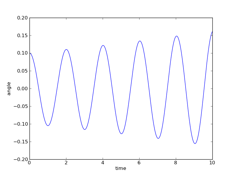
The Euler method gave "acceptable" results for our previous problems, but in this case of oscillatory motion the results are not acceptable. The problem originates in the truncation terms, or error, in the Euler method itself. This numerical error leads to changes in the energy of the system. Such errors existed in our previous problems, but they did not adversly affect the results. In this current problem we are calculating the motion for many dynamical times, allowing the errors to build up to noticable proportions. Furthermore, the oscillatory nature of the solution makes it easy to identify problems with conservation of energy: if the pendulum does not return to the same maximum amplitude, energy must have been gained/lost from the system.
We can quantify the accuracy of these methods by tracking the total energy of the system. By inspection, we infer that the total energy of the system is increasing with the Euler method (because the amplitude gradually increases), and constant with the Euler-Cromer method. The total energy of the pendulum is a sum of the kinetic energy and the gravitational potential energy:
where $h = L*(1-\cos(\theta))$ and $v = L*\omega$. Dropping constant terms we find that the total energy is proportional to:
Now that we have identified a problem with our solution, how do we fix it? In this case a very simple fix provides an algorithm that conserves energy exactly (to within machine roundoff). The Euler-Cromer method makes one slight change to the current algorithm, instead of using the angular velocity at the beginning of the time step, use the updated angular velocity to update the angle:
# Euler Method
   acceleration = (-g/L) * sin(theta[n])

# Euler-Cromer Method
   acceleration = (-g/L) * sin(theta[n+1])
Assignment: Submit your program using the Euler-Cromer method. It should produce a plot of angle versus time for at least ten oscillations, using both a small initial angle and a large initial angle. Does the frequency become larger or smaller than $\omega = \sqrt{g/L}$ when the small-angle approximation breaks down?