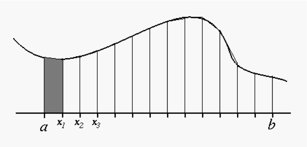
INTRODUCTION In the last lesson we looked at the left and right rectangular methods and saw how they both had numerical error compared to the exact result but that the error got smaller as the number of rectangles N increased. This suggests that if we simply use enough subintervals - i.e., we use a big enough N - and cross our fingers then the numerical error will be sufficiently small. But computing function values can sometimes be `expensive' i.e., it it can take a lot of time, so just making N big might mean the computer takes a long time before we get a result. We should try and be smart and attempt to find other ways to reduce the numerical error with more modest values of N.

Here's an idea: what if we combine two different methods, one which overestimates the integral and another which underestimates it, whose errors scale with the mesh size h in the same way, so that the error at leading order cancels. (The numerical errors at higher orders will not cancel so we haven't eliminated the numerical error entirely.) Plus if we pick the two methods we are combing carefully it's possible for two different methods to require essentially the same function evaluations. It's like we get an extra result for free! This idea of recycling function evaluations from one method and obtaining a second result from a different method for free is so good that you will see this idea used again and again in all sorts of numerical algorithms, not just numerical integration. This is today's `big idea'.

The Trapezoid Method We have already seen two methods which overestimate/underestimate the integral, the left and right rectangular methods. In this case the numerical errors (to leading order) are equal and opposite so all we have to do is add the two results together with equal weight of 1/2 to eliminate the error i.e., we average them. While averaging the results of the two rectangle methods certainly reduces the numerical error it would also appear to take us twice as long to compute the integral because we have to evaluate the function twice as many times. Why not just stick with one of the methods and double the value of N? But wait, that's not right! Except for the very first and very last intervals, the t on the the right hand side of a subinterval for the right-rectangular method becomes the value of t on the left hand side of next subinterval for the left-rectangular method! (Think about it). So if we cleave off from the expressions for the Riemann sum of the two methods the case where n=0 for the left-rectangle method and the n=N-1 from right-rectangle method and average the two we eventually obtain

Again, if we interpret this formula as being the `area under the curve' then what we are doing here is averaging the value of the function at the end points of the subintervals and then multiplying by the width. This is the same formula for the area of a trapezoid so the algorithm is known as the Trapezoid method.

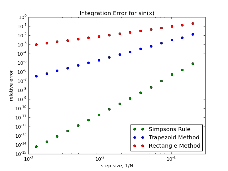
The trapezoid method computes just one more function value than either the right or left rectangular methods but the answer is much more accurate.

EXERCISE: Modify your Python code from the last assignment to again compute the integral of the function $\sin(x)$ between $x=0$ and $x=\pi/2$ for a given value of N, but now using the trapezoid method. Now how does the error scale with 1/N?

Simpson's Rule The other choice we had was to put the t's in the middle of the subintervals. You can go ahead and code up this choice too with just a small hack of your previous codes. Again it is a rectangle method but because the t's are put in the middle of the subintervals it is often known as the 'midpoint' method instead. And like the other two rectangle methods it will have a numerical error which we can reduce by increasing N. But if you go ahead and examine the numerical error of the midpoint method you will find that it does much better than either the right or left rectangular methods, in fact the numerical error is 50% smaller than the error of the trapezoid method and, more importantly, of the opposite sign. Again we have a pair of methods - the midpoint method and the trapazoid method - that have errors of opposite signs which scale with 1/N in the same way so if we combine the result from the midpoint method with weight 2/3 and the result from the trapezoid method with weight 1/3 the numerical error (at leading order) cancels. This weighted averaging of the midpoint and trapzoid methods is known as Simpsons rule (don't ask me why it's a rule and not a method). We will spare you the math of deriving it and simply state that:

In terms of area under the curve, what is going on here is we are approximating the function with parabolas. The function evaluations at the left-hand side, the right-hand side and the center of each subinterval are fit with a quadratic which is then integrated.

EXERCISE: Hack your previous codes to again compute the integral of $\sin(x)$ between $x=0$ and $x=\pi/2$ for a given value of $N$ using Simpson's rule. Now how close are your answers to the exact value for $N=2, 4, 8, 16$?

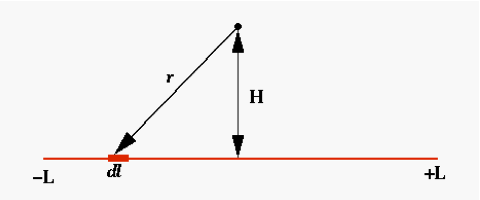
Assignment: Write a Python code that computes the electrostatic potential of a finite segment of charged wire of length 2L, at a height H=L above the center of the wire. The charge density along the wire varies as

Give your answer in units of $\lambda_0 / 4\pi\epsilon_0$. How might you test your program? Is there a similar problem you can solve analytically to provide a test of your code?

Beyond One Dimensional Definite Integrals Now you have a basic understanding of how to compute a definite one dimensional integral you can go out and read about how to do more complicated kinds of integrals: line integrals, surface integrals and the rest. They all use similar ideas of breaking the interval up, approximating the integrand in some way with a simple function, and then approximating the true integral as the integral of the simple function. But if you ever try these methods out you will find that beyond triple integrals the amount of time it takes to compute the result with reasonable accuracy can become excessive. Think about it, if we use, say, N=1000 for a 1-D integral to get 1000 subintervals, we would expect to generate 1,000,000 subintervals for a double integral (1000 subintervals in one variable, 1000 in the other), and 1,000,000,000 subintervals for a triple integral. In each subinterval we have to evaluate the integrand at least once and 1,000,000,000 evaluations of even a simple integrand will take a lot of time. For this reason multi-dimensional integrals beyond triple/quadruple integrals are typically evaluated using other techniques.