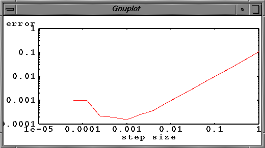
If we continue the error plot from the last lesson down to even smaller step sizes, we find some strange behavior if running with a 32-bit version of python:

There are a couple of unfavorable features of our numerical code that are illustrated in this error plot. First, the error term grows linearly with the step size, as expected from our derivation of the algorithm: The highest order term truncated in the expression for the first derivative varies linearly with the step size. Second, at small step size the error becomes both large and unpredictable. The first problem is a limitation of our simple numerical algorithm, the second is a limitation of the way the computer is representing numbers.
We can attack the first problem using a slightly more sophisticated finite-difference formula for the first derivative. Again we begin with the Taylor expansion, but now for both a step forward and a step backward.
Note that this equation is centered in x, in that it uses information from both a step forward and a step backward. The important feature of this equation is that the largest term in the series to be dropped now goes as the square of the step-size, h. Using this formula in our equation for radioactive decay we arrive at an algorithm for computing the number of nuclei a time $\Delta t$ in the future.
This formula presents a slight problem because it requires knowledge of the number of nuclei at two succesive times rather than just one. So to get started one needs both the initial number of nuclei and the number after one timestep. The simplest approach is to use our previous technique to get the number of nuclei at the first timestep, and from then on use the more accurate formula.
n[0] = 100.
n[1] = n[0] * (1.0 - dt/tau)
for i in range(1,steps):
   n[i+1] = n[i-1] - n[i]*2.0*dt/tau
Here we have used a slightly modified version of the range function where we specify both the starting and ending integers. Previously we had only used the ending integer in range, for which Python assumes the sequence starts with zero.
Alternatively, we can modify the algorithm slightly to avoid using two different times. Shifting this equation forward by $\Delta t$ we can rewrite it as
Now use a value of $\Delta t$ that is twice as big as the one used in the above formula.
The value at the midpoint of the timestep, $N(t+\Delta t/2)$ can be found using the original Euler method. This two-step algorithm is known as the second-order Runge-Kutta method. We will come back to this method later in the course.
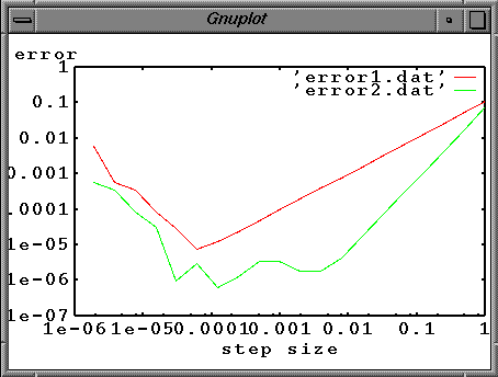
The plot below shows the output from the above program and the error data from the last lesson. The benefit of this slightly more complicated algorithm is evident. The slope of the error curve is approximately two, meaning that cutting the step size in half will decrease the error by four. Achieving a small error is much more efficient with the second-order algorithm.

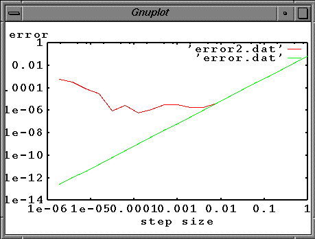
The other source of error is the limited ability of the computer to accurately represent numbers. Working in single precission (32 bits), real numbers are only accurate to about 6 decimal places: The computer cannot tell the difference between 1 and 1.00000001. In our current application, this roundoff error becomes larger than the truncation error at about 10-5 if run in single precision.
The easy way to reduce the roundoff error is to use double precision, such that numbers are represented by 64 bits rather than 32. In this case the accuracy of a given real number is extended to roughly 14 decimal places. A 64-bit version of Python is avaliable for linux, but not for Mac OSX.
EXERCISE: Estimate the accuracy of the IPython environment on your computer. Find a value of $\delta$ such that $(1.0 + \delta) - 1.0$ is no longer accurately computed.
The plot below shows output from a FORTRAN program comparing the Euler method with single (32 bit) and double (64 bit) precision.

Assignment: Modify your Euler error program from the last lesson to use the second-order Runge-Kutta method.