You should now have a working program that writes out the time and number of nuclei. Here is an example FORTRAN program that writes this data out to a file named "decay.dat":
program decay

implicit none
real time, tau, number, dt

open(12,file='decay.dat')

tau    = 5.0
dt     = 0.2
number = 100.0
time   = 0.0

do while (time < 5.0*tau)
 number = number * (1.0 - dt/tau)
 time   = time + dt
 write(12,*) time, number
enddo

close(12)

end
Before proceeding, make sure you have a working program that produces
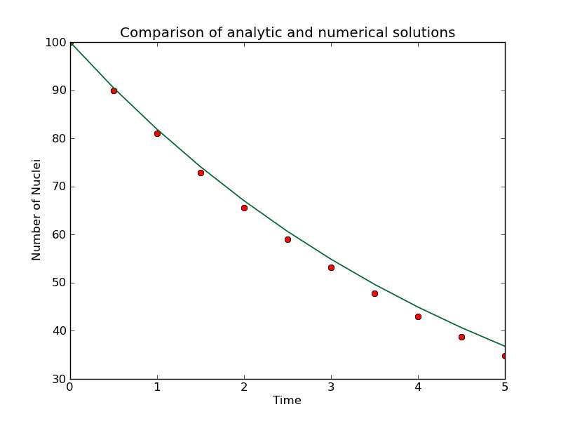
reasonable data. Using pyplot,
you should be able to make a plot
that looks like the one below. The red points are the data from
the numerical solution, and the green line is the analytic solution
as plotted by gnuplot.

Verification is the next, and most important, step. You must always be wary of falling into the trap of assuming the output of a program is correct. You should always ask yourself "does this make sense?" There are several ways you can verify that your program is working. The best is a direct comparison with the correct analytic solution. While that will work in this case, one does not often have this luxury. In the absence of an analytic solution, one can test the output as a function of step size or as a function of the input parameters.
A very crude test in this case would be to compare the output as a function of the mean lifetime of the nuclei. If the lifetime is shorter, the decay process should happen faster.
EXERCISE: Modify your program to query for the mean lifetime and then read the value input by the person running the program. Run your program for at least two different values of the lifetime. Do the results make sense? Does the run with a shorter lifetime have a more rapid decay?
A more rigorous test, and one that can almost always be implemented, is to compare the output of a method for different values of the step size. From our analysis in the last lesson, the accuracy of our crude method improves as the size of the timestep decreases.

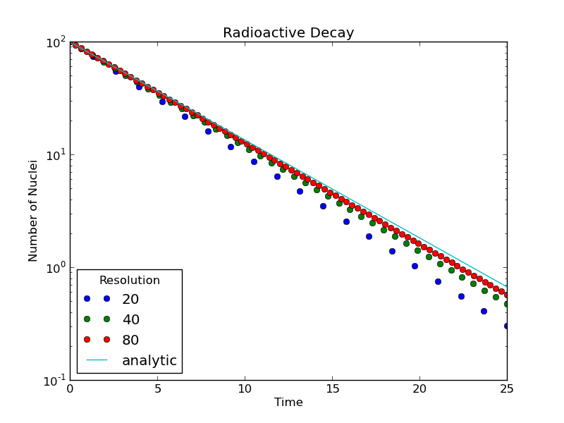
In our decay program, one can plot the output for several different runs and visually see that a smaller timestep provides for a more accurate solution, in the sense that the output more closely approximates the analytic solution. Also note that the numerical solutions start to converge onto the same line as the timestep gets smaller. This brings up the point that one is almost always dealing with an approximate solution; the question is not "do we have the right solution," but rather "is the solution accurate enough?"
We can quantify this analysis of the numerical error with the goal of producing an error plot in which the error is plotted as a function of the step size. The first question is how do you define the error? If you know the analytic solution this is obvious. If you do not have this luxury, you can infer the exact numerical solution by plotting the answer as a function of step size and extrapolate to zero step size.
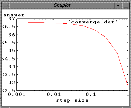
A convergence plot can be made by recording the numerical value of the number of nuclei at a specific time for several values of the step size. Plotting this value as a function of step size, one could extrapolate down to zero step size. This does not guarantee the correct answer, but if the numerical method is working correctly it should give a good approximation. The plot below shows the value of the numerical solution at a time of one lifetime (which should be 100*exp(-1)=36.7879) as a function of the step size. As the step size is decreased, the numerical solution converges on the correct value.

To produce an error plot, we want to run our decay program to a specified time (e.g., one mean lifetime) and output both the step size and the error. In this case it is useful to define the relative error as the difference between the analytic answer and the numerical answer divided by the analytic answer.
We could run our program several times to generate the data for the convergence plot, or we could let the program do the work. Ultimately we want to plot error versus stepsize, so we want our program to generate arrays of each that we can pass to the plot routine.
Its always useful to start from an existing, working program, so go back to your program for calculating radioactive decay, and instead of having it plot N(t), have it run to a fixed time and compute the error at that time. Note that this means you don't necessarily have to store arrays of n, t. In this case, your simplified program should look something like:
from matplotlib.pylab import *

endtime = 5.0   # end time of simulations
tau     = 5.0   # mean lifetime
N0      = 100.0 # initial number of nuclei

answer  = N0 * exp(-endtime/tau)   # analytic answer

steps   = 10    # number of iterations
t  = linspace(0.0,endtime,steps)
dt = t[1]
N[0] = N0

for i in range(steps-1):
   N[i+1] = N[i] * (1.0 - dt/tau)

error = (answer - N[steps]) / answer
print error, dt
In order to generate data at different step sizes, write an outer loop that changes the number of steps used in each calculation:
for j in range(10):
  steps = steps * 2   # increase the number of steps each cycle
  ... code to compute error ...
  error[j] = (answer - N) / answer
  stepsize[j] = dt
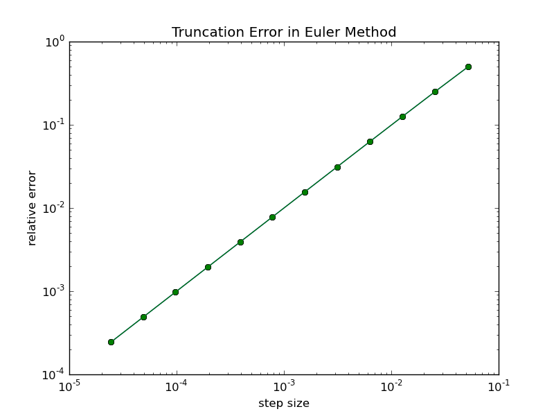
Plotting the results of this program gives us an error plot that illustrates the rate at which the numerical error decreases with step size. Note that this type of plot is typically a log-log plot because the size of the error spans orders of magnitude. To generate a log-log plot, use the commands
plot(error,stepsize)
xscale('log')
yscale('log')
show()
The slope of the error curve on a log-log plot gives the order of accuracy of the method. If the slope is unity, then the error scales linearly with the step size. If the slope is two, then the error scales as the square of the step size. In such a case dropping the step size by a factor of two reduces the error by four; clearly an advantage over the linear scaling we see here.

Assignment: Submit a code that produces an error plot like the one above.