Radioactive Decay of unstable nuclei, like ²³⁵U, is a statistical process in the sense that a given nuclei has a probability of decaying at a particular time, but one cannot know exactly when that nucleus will decay. Instead, one can define the mean lifetime of a nucleus.

The mathematical equation describing this decay process is a first order differential equation. If N(t) is the number of radioactive nuclei at a time t, the evolution of N(t) is given by:

The solution to this equation is straight forward:

Our task now is to construct a numerical solution to the decay equation. While we already know the exact analytic solution, constructing an approximate numerical solution is not just a trivial excercise.

To construct the numerical algorithm we replace the derivative with a finite difference approximation:

Rearranging terms, we arrive at an equation describing the evolution of N(t), namely we can now compute N(t+dt) from knowledge of N(t). From this we can step forward in time in steps of dt.

We can also arrive at this equation using a Taylor series expansion:

The difference between the infinite series above and the previous equation involves terms that are quadratic or higher in the step size. Hence, provided that $h$ is sufficiently small, these higher order terms can be safely neglected. These higher order terms that are dropped from the equation used in the numerical algorithm is referred to as the truncation error.

EXERCISE: Compute by hand the population of radioactive nuclei at one second intervals assuming an initial population of 100 and a mean lifetime of 5 seconds. (Use a calculator if necessary, but no programming.)

The accuracy of this numerical solution clearly depends on the size of the chosen timestep; a larger timestep produces larger error. Because our model equation has an analytic solution, we can write down explicitly the magnitude of the numerical error as a function of the value of the timestep.

EXERCISE: Use the series expansion of the exponential function to compare the analytic and numerical solutions after one timestep. Express the difference between the analytic and numerical solutions as a function of the size of the timestep.

Programming this numerical algorithm into a working computer code is the next step in our process. Before writing down some code, you should do two things: (1) think carefully about what you need from the program, i.e., what output will you need in the end, and (2) list the logical steps that the program will have to step through to arrive at the desired result.

EXERCISE: Sketch out your program. Define exactly what you want the program to give you. What will you do with this data? List the steps that you went through in the previous exercise to compute the evolution of N(t). Be as specific as you can.

Now turn these steps into a program utilizing a loop to step through 10 time steps from a time of zero to a final time of 5 (one lifetime).

When writing a more advanced program it becomes important to be able to tell the computer to execute different commands in different situations and to repeat the same command many times (without us having to write it all the times). Let us start with the repetition of the same command many times. This is called a cycle. The few lines below show how to write a program that computes the sum of the first 100 integers and prints it on the screen.

thesum = 0
for i in range(101):
    thesum = thesum + i
print 'the sum of the first 100 integers is: ', thesum

A few thigs are worth discussing. We use the command for at the beginning of the cycle. We then use the variable i as the one that we want to increase at every step and we define the range in which we want i to range with the range command. We end the line with a :. In the following line (or lines if we want to repeate more than one instruction) we write the instruction that needs to be repeated once for every passage. Note that the instructions that are part of the cycle are indented. In python there is no explicit way to close the loop. A loop is closed when the instructions are not indented. In the above example, the print command is executed only once after the cycle is completed.

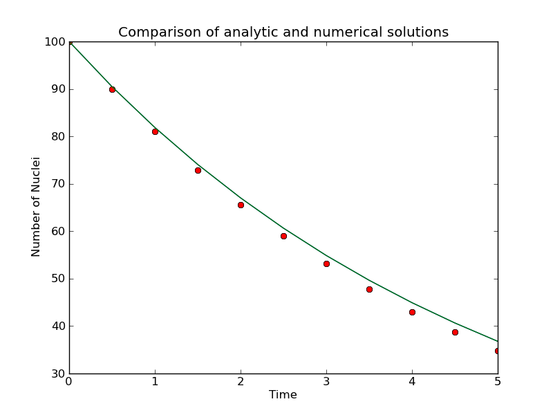
Finally, use the plot() routine to plot N(t) from your data to generate something that looks like:

Here the exact analytic solution is plotted on the same graph, providing a quick visual check on the accuracy of the numerical solution.

ASSIGNMENT: Submit your working radioactive decay program that plots the results of your numerical solution as points along with the analytic solution as a continuous line.