Computational Physics is, in the simplest definition, doing physics with computers. But as in most of today's high-tech society, computers are used to do virtually everything in physics. An experimental physicist might use a computer to gather data or design a piece of equipment, a theoretical physicist might use a computer to evaluate complicated integrals or graph an analytic function, and all physicists use computers to communicate the results of their work.
In a more restrictive definition, computational physics refers to the work done by a growing fraction of physicists who use computers as their primary investigative tool. Building on a mathematic or statistical description of nature, a computational physicist develops a computer model of a given physical process or phenomenon.
NC State University is an international leader in computational physics, with strong research programs in solid state physics and astrophysics. Here are some examples of recent research projects here at NC State:

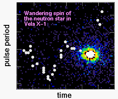
 Some of the brightest sources of X-rays in the sky are pulsed sources, with
the X-rays flashing on and off with periods ranging from fractions of a second
to several minutes. These sources are identified with binary stars in which a
normal star is transferring gas onto a neutron star companion. The pulse
period associated with the rotation period of the neutron star, which implies
that any change in the pulse period represents accretion of angular momentum.
The flow of gas from one star onto the neutron star is a non-linear,
time-dependent, multi-dimensional process that is NOT going to be solved with
pencil and paper. In the computational physics approach a detailed numerical
model is developed to study the dynamics of gas flow, and in particular, what
processes determine how much angular momentum might be accreted onto a neutron
star.

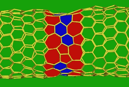
One of the most exciting new materials discovered in recent years is the carbon nanotube, a narrow tube made of linked carbon atoms with a diameter of only a nanometer. These tubes have extremely high tensile strength and can conduct electricity. These tubes may in the very near future replace wires and switches for electronic devices that you use every day! The image below is from a molecular dynamics simulation of this carbon structure. The yellow lines represent the carbon-carbon bonds, and the distortions highlighted by red and blue are caused by impurities in the carbon lattice.


We will explore many different subfields of physics this semester, building on your basic knowledge of mechanics to investigate chaos, the three-body problem, waves, random motion and diffusion...Show examples of these...
There are several components that make up computational physics:
- Physics
- Numerical Methods
- Computer Programming
- Data Visualization
- Scientific Communication
Physics is the study of nature, in its most basic form. Mathematics is the language of Physics. We use mathematical equations to transcribe the physical laws that define the way our Universe works. Often these equations are too complex for direct solution, and so we turn to numerical methods.

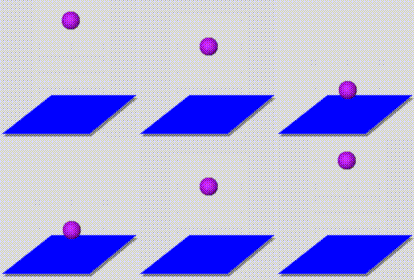
Consider the simple phenomenon of a bouncing ball. Except for the interaction of the ball with the floor, the only physics involved is gravitational acceleration. The mathematical formula describing this motion is perhaps the (second) most famous equation: F=ma, where a is the (constant) acceleration due to gravity.
Numerical Methods are algorithms, or "recipes", that are designed to accomplish a given task. There are a multitude of different numerical methods employed by physicists, of which we will use only a few of the most common. These will include numerical integration, finite-difference techniques to solve differential equations, root-finding, fast Fourier transforms, spectral methods, random methods, etc.
A common numerical approach to differential equations like F=ma is to rewrite the derivatives in terms of finite differences. In this case we first turn F=ma into two separate first-order differential equations, F=mdv/dt and v=dx/dt. Then the derivatives are written as:

These equations can then be rewritten to give the position and velocity at a time t+dt in terms of the position and velocity at a previous time t. By stepping forward in time in steps of dt, one can calculate the functions v(t), and x(t).


Programming is the process of transcribing the appropriate numerical method into a set of instructions that the computer can understand. Although it may seem like the least important piece of computational physics, this skill is essential. There are several choices one can make regarding a programming language. One choice is a software package like Maple or Mathematica. These tools can be very powerful and easy to use, but they cost money, they are not always practical, and they are in general very inefficient. An alternative is to use a standard high-level programming language. These are standardized languages available on most computers (we're not talking Microsoft here). Two standards are FORTRAN and C/C++.
- FORTRAN
- This language was developed many moons ago for the purpose of scientific computing, hence it should be of no surprise that it is still widely used today. FORTRAN has evolved significantly over the years, resulting in a new standard, FORTRAN 90 (The last standard was FORTRAN 77). gfortran is the standard open-source compiler for FORTRAN, although an independent open-source project, g95 provides an alternative.
- C++
- This is a much more "modern" language, capable of much more than FORTRAN can handle. However, most of these additional capabilities are not necessary for the type of scientific computing that arises in computational physics. On the other hand, if you will be doing more than just scientific programming in your future, learning C++ rather than FORTRAN may be an investment in the future. gcc provides the standard open-source compiler for C and C++.
- Python
- We will use Python in this course, as it provides a easy introduction to programming and it provides a much more complete computing environment. For example, we will make extensive use of the matplotlib functionality to integrate plotting into our numerical computations. You can access a Python tutorial here. We will use the Enthought distribution in our class, which combines several packages (numpy, scipy, matplotlib) useful for scientific computation into one software package.
The following program executes the above numerical algorithm 300 times, stepping the trajectory of the bouncing ball through several bounces.
from matplotlib.pylab import *

# Use the Euler method to compute the trajectory of a bouncing
# ball assuming perfect reflection at the surface x=0.
# Use SI units (meters and seconds)

steps = 300     # number of time steps computed
endtime = 3.0   # end time of simulations
g = 9.8         # acceleration due to gravity

# create 1D arrays of length steps+1 for time (t), position (x), velocity (v)

t = zeros(steps+1)
x = zeros(steps+1)
v = zeros(steps+1)

# initialize variables at time = 0.0

x[0] = 1.0
v[0] = 0.0
t[0] = 0.0

dt = endtime / float(steps)

for i in range (steps):
   t[i+1] = t[i] + dt
   x[i+1] = x[i] + v[i]*dt
   v[i+1] = v[i] - g*dt
   if x[i+1] < 0.0:    # if ball is below surface, reflect it
      x[i+1] = -x[i+1]
      v[i+1] = -v[i+1]

plot(t, x)
show()
Data Visualization is an essential tool in computational physics. The output of a computer program like the one above is typically a bunch of numbers, perhaps billions of them. If one is to use these numerical tools to learn about the world around us, the physicist must be able to extract useful information from this mountain of numbers. There are many different ways to visualize data with a computer, as we have seen earlier in this lesson. We will restrict our attention in this course to one-dimensional data sets, i.e., X(t) as in our sample problem. We will use the Pyplot routines in matplotlib. Here is a tutorial for Pyplot.

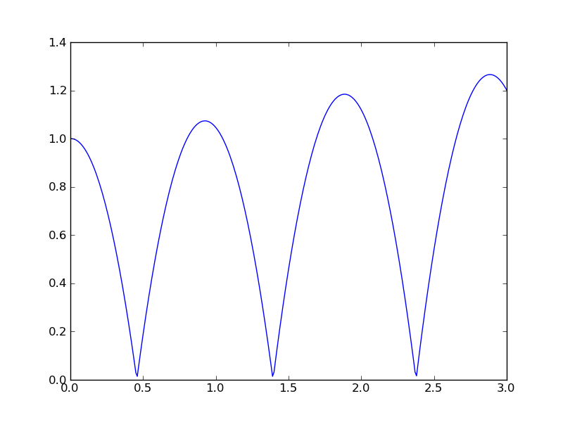
Here is the output from
the Python program shown above, showing the position of the bouncing ball
as a function of time. Does this look correct?
Communication of results is an often neglected component of physics education, but in the real world it is one of the most important skills a person can posess. In this course we will evolve away from short numerical answers (i.e., the answer is 42) and towards comprehensive solutions. By the end of the semester projects will be turned in as complete scientific papers.

Your first activity for the semester is to log into your computer, fire up IPython, and learn a little about Python coding...
For more practice, and a more complete introduction to Python, spend some time with the python tutorials at Code Academy.
